
DOC 03SIMULATION CONTENT
Sensors
LEVIATHAN simulates optical, acoustic, navigation and oceanographic sensors at two levels of rigour. Analytic models are fast, configurable and broad. Canonical measurements are computed from immutable World snapshots and carry full ground truth.
Two levels of sensor model
| Analytic sensors | Canonical measurements | |
|---|---|---|
| Sensors | 21 models in the live catalogue: cameras, sonars, positioning, navigation, oceanographic | RGB camera (PerceptionFrame), forward-looking imaging sonar, four-beam DVL, strap-down IMU, pressure, magnetometer, USBL |
| Input | A pose, an environment and simplified scene geometry | An immutable snapshot of a committed World state |
| Scene geometry | Seabed, obstacle footprints and labelled primitives | The frozen canonical scene: seabed triangles, structure meshes and dynamic rigid bodies |
| Time | Floating-point time within a rollout | Integer-nanosecond schedules, exact ticks only |
| Noise | Per-sensor Gaussian noise, reproducible with a seed | Off unless configured; keyed draws, independent of batching |
| Identity | None | Content-addressed record with array digests and provenance |
| Used by | Viewport payload, Dashboard panels, scenario rollouts, learning environments | Perception, datasets, camera–sonar ground truth, the localization estimator |
The Viewport payload
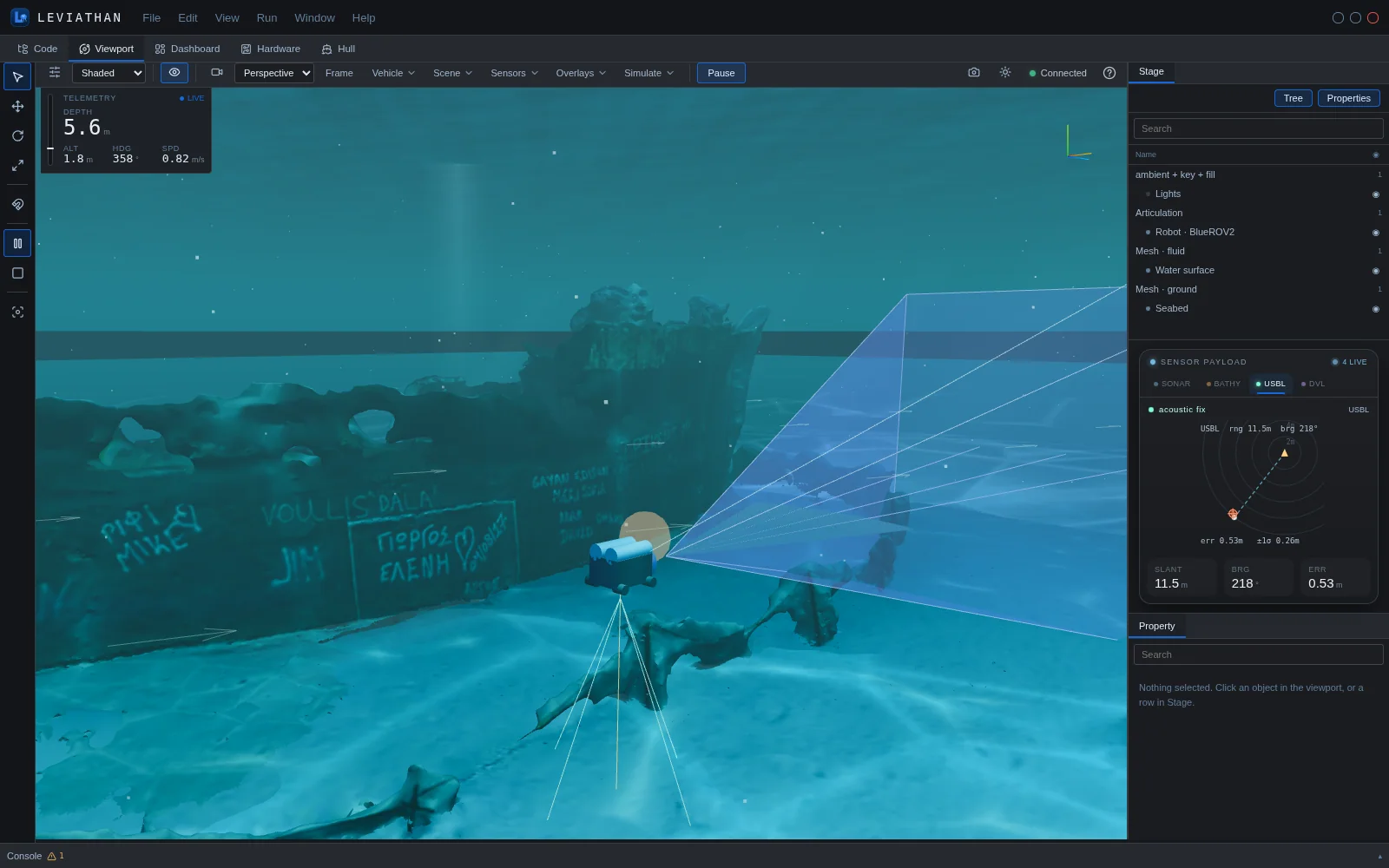
The Viewport's Sensors menu toggles thirteen sensors on the current vehicle: DVL, Sonar, Camera, LiDAR, Bathy, USBL, LBL, GPS, IMU, Depth, Compass, CTD and ADCP. Acoustic footprints are drawn in the scene. Live readings appear in the Sensor payload card in the Stage dock, one tab per sensor that has a view.
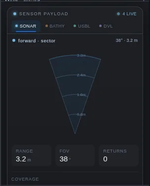 Sonar · forward sector, range, FOV, returns
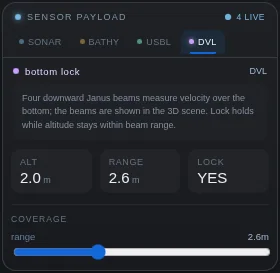 DVL · altitude, beam range, bottom lock
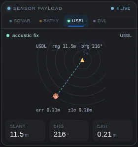 USBL · slant range, bearing, fix error
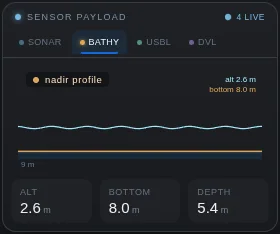 Bathy · nadir profile, altitude, depth
Vision
| Sensor | Measures and outputs | Key parameters | Character |
|---|---|---|---|
| RGB camera (PerceptionFrame) | Clean, underwater and sensor-response images; range, z-depth, normals, semantic and instance labels per pixel. OpenCV optical frame | resolution, hfov, max range, distortion k1–k3 p1 p2, water, ambient, exposure | Canonical Camera and optics |
| Underwater camera | Contrast loss with range: direct signal attenuated as e−cz plus a veiling backscatter that grows with range | attenuation c = 0.3 1/m, backscatter B∞ | Analytic |
| Stereo camera | Range from disparity, z = f·b/d; range error grows with z²; optional flat-port refraction bias | baseline 0.1 m, f 600 px, disparity noise 0.2 px | Analytic |
| Depth camera | Per-point range from a time-of-flight or structured-light sensor; noise grows linearly with range; usable range capped by water clarity | noise 0.02 m + 1 %, max 10 m | Analytic |
| Scanning LiDAR | Blue-green laser range scan: an azimuth × elevation point cloud in world XYZ, range capped by water clarity | 16 × 8 rays, max 30 m, noise 0.02 m + 1 % | Analytic |
| Thermal camera | Per-pixel temperature, assigned by the label of the surface seen, against an ambient background; not a radiative infrared render | 64 × 48 px, hfov 80°, ambient 10 °C, noise 0.05 °C | Analytic |
| Event camera (DVS) | ON/OFF events where log-brightness changes beyond a threshold between two poses | 64 × 48 px, contrast threshold 0.15 | Analytic |
| Optical-flow camera | Dense image-plane flow from ego-motion only | 64 × 48 px, dt 0.1 s | Legacy superseded by canonical optical flow |
The Viewport's live camera feed shows RGB, depth or segmentation views rendered by the 3D view for display. Scientific camera data comes from the PerceptionFrame capture in the same panel; see Camera and optics.
Acoustics
| Sensor | Measures and outputs | Key parameters | Character |
|---|---|---|---|
| Imaging sonar (canonical) | Range × azimuth relative return with per-cell primary and top-K contributors, validity codes and ground truth. Sensor FRD frame | frequency, azimuth FOV, elevation aperture, beam pattern, range window, bins, elevation samples, K | Canonical Imaging sonar |
| Acoustic image sonar | Range × azimuth intensity image with elevation spread, time-varied gain and speckle (Dashboard Imaging sonar panel) | 256 beams, 256 bins, max 30 m | Analytic |
| Mechanical / profiling FLS | Nearest-obstacle range per bearing across a horizontal fan | 64 beams, FOV 120°, 0.1–30 m | Analytic |
| Side-scan sonar | Port and starboard slant range and first-order Lambertian backscatter per across-track beam; stacked into a waterfall | 64 beams, 10–80° off vertical, max 100 m | Analytic |
| Multibeam / echosounder | Per-beam slant range to the seabed across a swath; travel-time range biased by the sound-speed profile | 32 beams, swath 120°, max 100 m | Analytic |
| Altimeter | Single-beam slant range to the seabed, optionally with sound-speed bias | noise, sound-speed profile | Analytic |
| ADCP | Water velocity in range bins along the vertical, looking down or up | 20 bins × 2 m, blank 0.5 m, max 60 m | Analytic |
| USBL (canonical) | Slant range, azimuth, depression and position fix of the vehicle's transponder from a declared transceiver, using the analytic model's sound-speed bias; refused beyond its maximum range | transceiver position, range and bearing noise, sound speed, max range | Canonical |
| USBL | Slant range and bearing (azimuth, depression) from a known transceiver; range error grows with range, bearing error is constant in angle | range and bearing noise, sound speed 1500 m/s | Analytic |
| LBL | Ranges to three or more seabed beacons, trilaterated horizontally with depth from the pressure sensor; geometry sets the dilution of precision | range noise, sound speed | Analytic |
Further acoustic tools appear as Dashboard panels: side-scan survey waterfalls with gain, time-varied-gain flattening, ground-range correction and per-ping A-scan inspection, multibeam bathymetry strips over a choice of sound-speed profiles, echograms, beacon networks and acoustic communications. See Dashboard.
Navigation and inertial
| Sensor | Measures and outputs | Key parameters | Character |
|---|---|---|---|
| DVL (canonical) | Four Janus beams cast against the full canonical scene; along-beam velocities and a least-squares bottom-track velocity in the sensor frame, with residual; optional water track | beam angle, beam azimuths, min/max range, noise, dropout | Canonical |
| DVL | Bottom-locked body velocity within a maximum altitude | beam angle 30°, max altitude 50 m | Analytic |
| IMU (canonical) | Specific force and angular rate at the mount, including lever-arm effects, from the dynamics' own acceleration; reported bias | noise density, bias instability, rate random walk | Canonical |
| IMU | Body-frame specific force and angular rate | accel and gyro noise | Analytic |
| Pressure (canonical) | Absolute pressure at the sensor point below a declared free surface; refused when no surface is declared or the sensor is out of the water | water density, atmospheric pressure, bias, noise [Pa] | Canonical |
| Pressure / depth | Hydrostatic pressure p = patm + ρgd | ρ 1025 kg/m³, noise [Pa] | Analytic |
| Magnetometer (canonical) | Three-axis field vector in the sensor frame from a declared local field, with hard-iron offset, optional timed external disturbance and noise | declination, inclination, intensity [nT], hard iron, noise | Canonical |
| Magnetometer / compass | Body-frame geomagnetic field with hard-iron offset and soft-iron distortion; yields heading | declination, inclination 60°, noise | Analytic |
| GPS | Horizontal fix only at or near the surface; no fix when submerged, no depth | noise 2.5 m, max fix depth 0.5 m | Analytic |
| Surface radar | X-band surface-search radar for surface craft: nearest contact per bearing over a 360° sweep | 128 beams, 2–500 m | Analytic |
Canonical DVL
Beam i points along bi = [sin a cos φi, sin a sin φi, cos a] in the sensor frame. Here a is the beam angle from the sensor's down axis and φi the declared beam azimuths, by default forward, aft, starboard and port. Each beam is cast against the same frozen scene the camera and sonar see, so structures and moving bodies block beams as the seabed does. The along-beam velocity is the relative velocity between the transducer and the surface point the beam hits:
A beam loses lock when no surface lies within its range window, or when it reaches the sea surface first. With fewer than three valid beams there is no solution. Three beams determine the velocity exactly; four give a least-squares solution and an RMS residual. Water track uses the current-relative velocity, with the current uniform over the vehicle. It has no range limit or scatterer model, and the record says so.
Canonical IMU
The IMU uses the committed state exactly, never a finite difference: orientation, twist and the dynamics' own acceleration. At a mount offset r:
At rest and level, the specific force is [0, 0, −g]. If the provider has no acceleration, the gyroscope is still reported and the accelerometer is marked unavailable rather than invented. Noise follows IEEE Std 952-1997 terms: white noise from a noise density, bias instability as a first-order Gauss–Markov process, and rate random walk, using the schedule's actual sample interval. The bias at sample n is evaluated in closed form, so it is identical whether a sample is produced alone or in a batch, and it is reported beside the measurement as ground truth.
Canonical pressure, magnetometer and USBL
These three measure what the device measures, not a convenient derived quantity. The pressure sensor reports absolute pressure in pascals, not depth. The magnetometer reports a field vector, not a heading. The USBL reports range and bearings and the resulting fix. Each takes its geometry from the vehicle's declared mount, so lever arms count. Each uses declared environmental inputs: the free-surface level, the local magnetic field and the transceiver position, each with its source. Measurements that cannot be made are refused with a reason, for example a pressure sensor above the surface or a USBL beyond range. Truth is reported beside each measurement for scoring only.
The magnetic field is one constant vector for the scene, not a spatially varying Earth model, and soft-iron distortion is not modelled. Pressure uses constant-density hydrostatics, with no drift or temperature effects.
From sensor to workflow
Canonical sensors sample on their own declared schedules from committed World states. A sensor rig turns each measurement into a sensor packet: a small, typed, immutable view carrying the vehicle, sensor, frame, integer timestamp, validity, the measurement's identity and its payload. Packets from different sensors are interleaved in a deterministic time order without being forced onto a common timestamp. A refused measurement stays refused all the way down, so consumers never see a fabricated value.
Packets feed the localization estimator. The same measurements are written to datasets (Synthetic data and export) and are the inputs to the perception algorithms.
Environmental
| Sensor | Measures and outputs | Units |
|---|---|---|
| CTD | In-situ temperature, practical salinity, hydrostatic pressure and local sound speed (Mackenzie 1981) through a mixed-layer, thermocline and deep profile | °C, PSU, Pa, m/s |
| ADCP | Binned water-column current profile; listed under Acoustics | m/s |
Noise and ground truth
| Aspect | Analytic sensors | Canonical measurements |
|---|---|---|
| Default noise | Most analytic defaults are zero; GPS, depth camera, LiDAR, stereo and thermal have non-zero defaults | Off unless configured |
| Noise model | Zero-mean Gaussian per reading or beam; some sensors grow with range | Specified per sensor (above); keyed by seed, sensor, sample and channel |
| Ground truth | The true vehicle state from the same rollout | Per pixel, per cell or per beam: hit geometry, identity and validity, plus the true state in the snapshot |
- Analytic sensors see simplified geometry: a seabed function, obstacle footprints and labelled primitives, not the detailed scene meshes.
- The canonical sensor set is the camera, imaging sonar, DVL, IMU, pressure sensor, magnetometer and USBL. GPS, side-scan, multibeam, LiDAR and the other models are analytic only.
- In the canonical catalogue, the built-in production vehicles declare a front camera only. The sonar and navigation sensors are declared on the catalogue's reference vehicles, which are labelled test and reference models.
- Sensor timing models exact sampling instants. Exposure time and transport latency are not part of canonical measurements.